CASE STUDY 2026
SLIDERS: Steering Image Retrieval with Sparse Visual Features
A patch-level image retrieval system in which sparse visual features become named controls for changing the ranking at query time.
Most image retrieval systems answer one question: which images are closest to this query?
SLIDERS asks a second one: closest in which visual direction?
A normal embedding search compresses the query into a vector and returns its nearest neighbours. That works well when the desired notion of similarity is already encoded in the original query. It is less useful when the user wants to preserve the general image while changing one property, such as stronger yellowing, darker lesions, a more prominent vein or a different edge pattern.
The project turns those properties into controls. A user uploads an image, inspects the visual features discovered by the model and changes their strength through sliders. The query is modified before retrieval, so the ranking changes because the representation itself has moved, not because a text filter was applied afterwards.
The current implementation focuses on local visual evidence. Instead of representing an image with only one global token, it preserves its patch descriptors, learns sparse features from those patches and performs retrieval through late interaction.
From an image to 256 visual regions
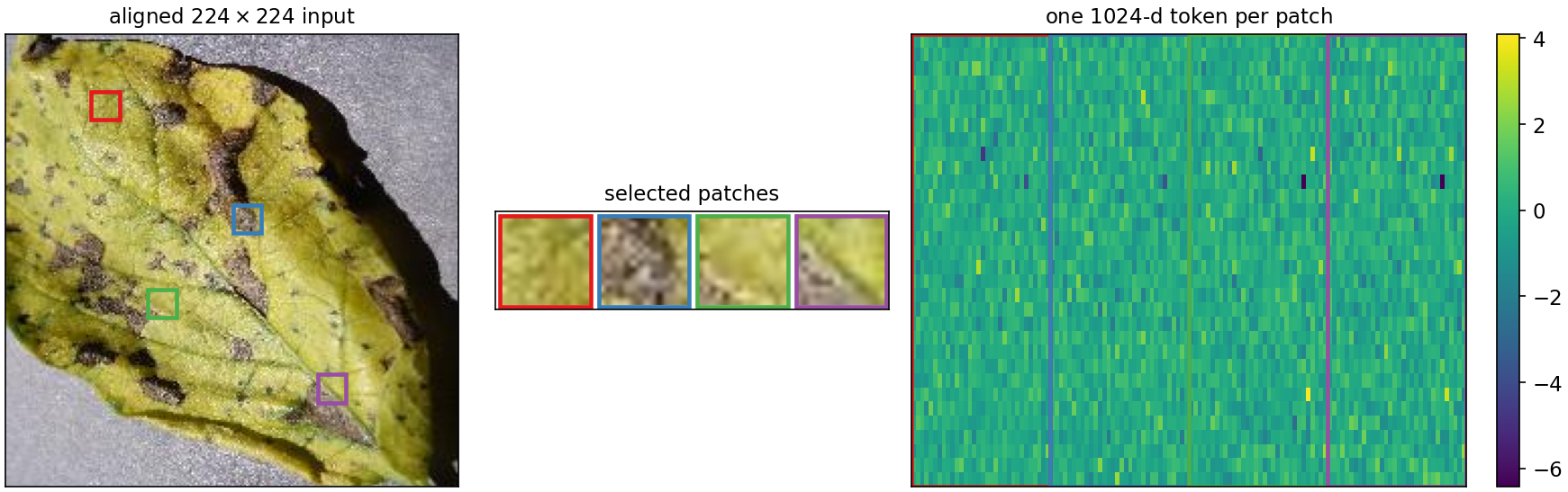
The visual backbone is the register-token variant of DINOv2 ViT-L/14. Every input is resized, centre-cropped to 224 × 224 and divided into a 16 × 16 grid. The result is 256 patch tokens, each with 1024 dimensions.
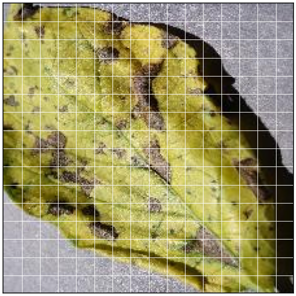
image
  -> DINOv2 ViT-L/14 registers
  -> 256 patch tokens
  -> tensor with shape [256, 1024]
Using patches rather than a single CLS embedding changes what the rest of the system can learn. A whole-image vector may encode that an image contains a diseased leaf, but it does not preserve an explicit correspondence between a feature and the region that caused it. Patch tokens retain that spatial link.
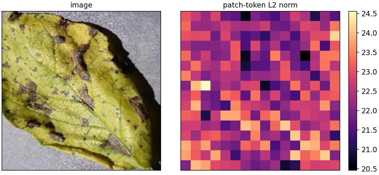
The register variant matters because standard Vision Transformers can produce a small number of unusually high-norm patch activations that do not correspond cleanly to visible content. A sparse model may treat those artefacts as meaningful features. Register tokens absorb much of that behaviour, leaving the spatial tokens more suitable for dictionary learning.
The patch corpus is written as a memory-mapped array rather than loaded entirely into RAM. Each row is associated with an image identifier, while metadata records the grid shape and preprocessing configuration.
Learning a sparse visual dictionary
The central model is a Sparse Autoencoder trained directly on the DINOv2 patch tokens. Its hidden layer is deliberately overcomplete:
1024-dimensional patch token
        -> encoder
8192-dimensional sparse code
        -> decoder
1024-dimensional reconstruction
Formally:
h = ReLU(W_enc x + b_enc)
x_hat = W_dec h + b_dec
The objective is not compression. The hidden layer is eight times wider than the input because the model needs enough capacity for individual units to specialise. A feature can remain inactive for most patches and respond only to a specific pattern.
I used a TopK constraint with L0 = 40. For every patch, only the forty strongest activations survive; the other 8,152 units are set to zero before decoding.
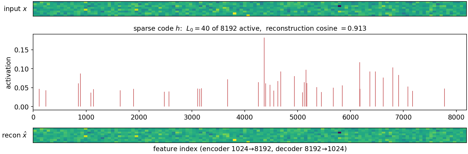
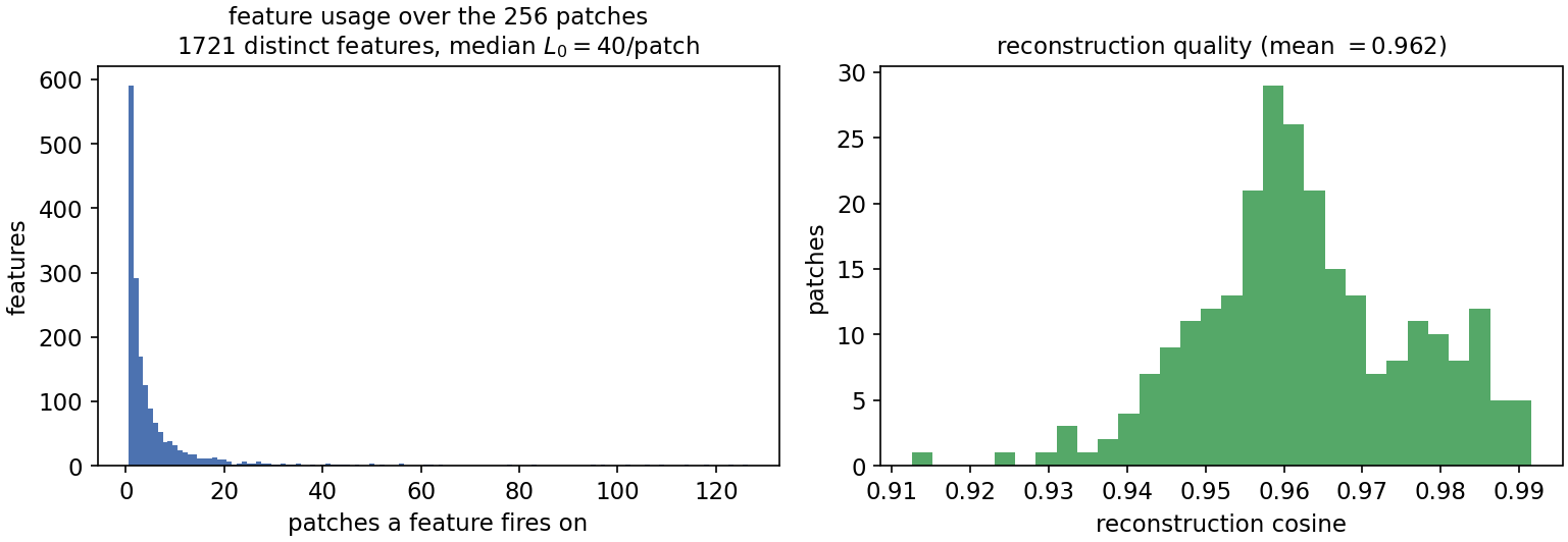
On one representative patch, the sparse code reconstructed the original token with a cosine similarity of 0.913 using only 40 active features. Across the 256 patches of the inspected image, the mean reconstruction cosine was approximately 0.962. The same image activated 1,721 distinct features in total, but most of them fired on only a small number of patches.
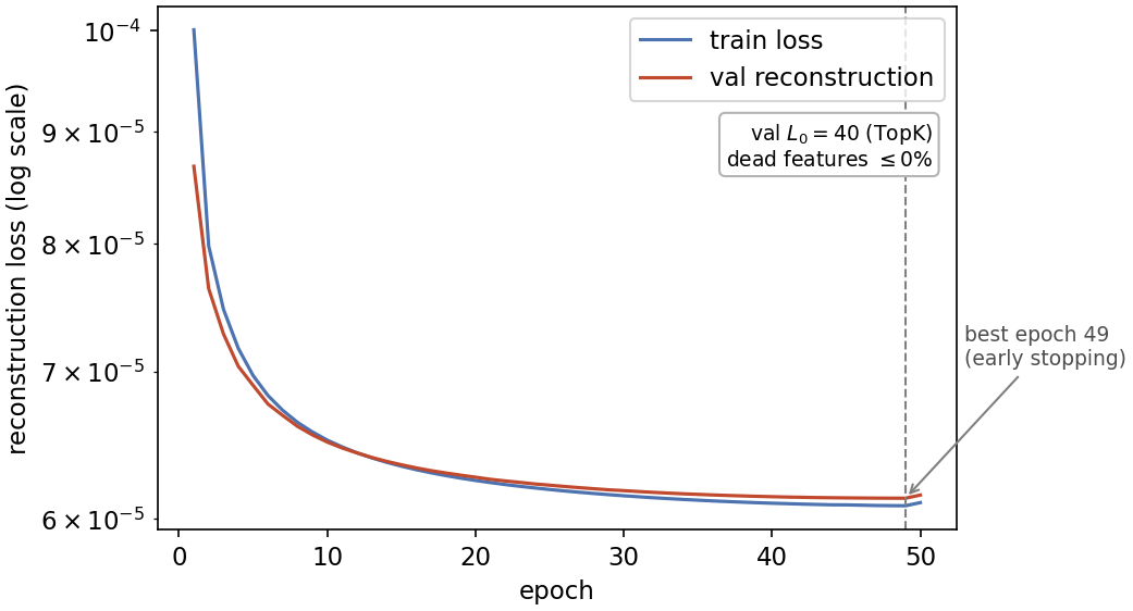
Training and validation reconstruction losses decreased together. Early stopping selected epoch 49, and the dead-feature fraction remained at zero. Decoder columns are normalised after optimisation, while features that remain inactive for too long are recycled using residual directions.
The decoder is more than a reconstruction matrix. Each column is a unit-length direction in the original 1024-dimensional DINOv2 space. Those columns are the actual slider directions.
A feature needs evidence before it gets a name
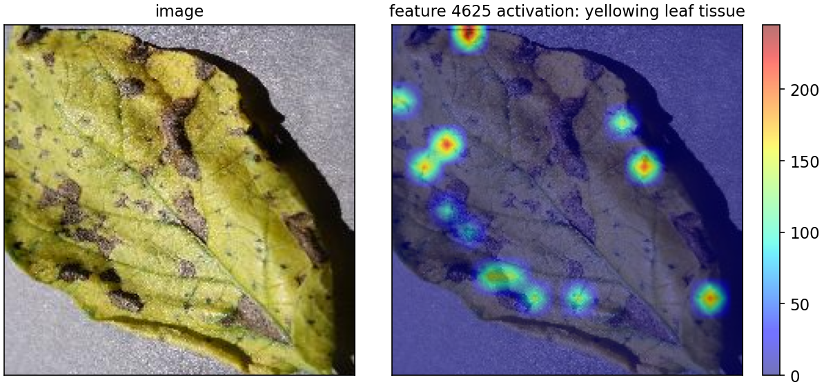
An index such as feature 4625 is useful for debugging, but not for an interface. Naming therefore became a separate pipeline rather than a cosmetic step.
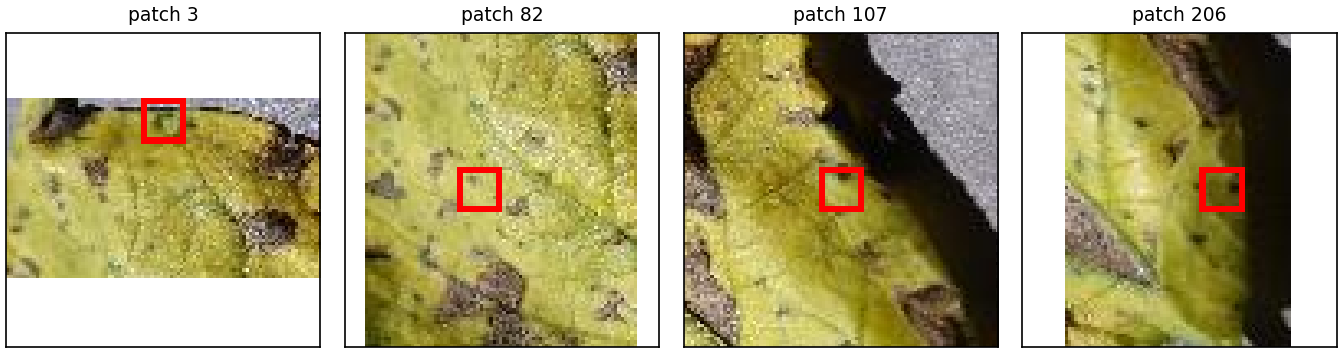
For every candidate feature, the system searches the patch corpus for high-activation and low-activation examples. It extracts a larger context crop and marks the active cell instead of sending an isolated 14 × 14 patch to the Vision-Language Model.
The VLM is shown contrasting groups: patches where the feature activates strongly, patches where it is weak or absent, and the corresponding image context. It is asked for the visual property that separates those groups.
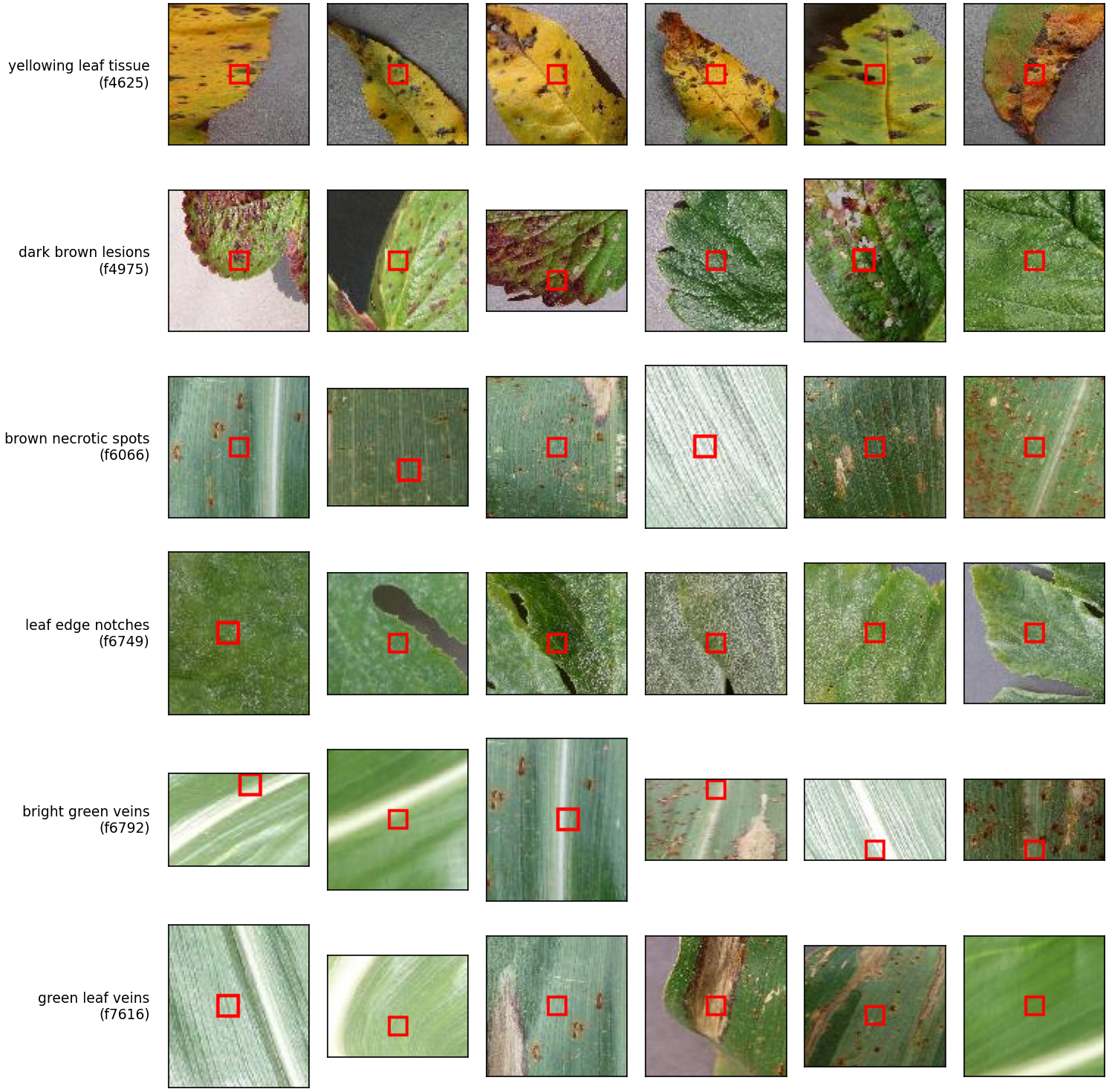
A second pass checks whether the proposed label is actually supported by the examples. Weak or generic names can be rejected. This process produced features such as yellowing leaf tissue, dark brown lesions, brown necrotic spots, leaf edge notches, bright green veins and green leaf veins.
The local crops make the evidence inspectable. They show the active patch in context and make it easier to determine whether a unit responds to the intended visual property or to a nearby artefact.
A broader feature gallery shows whether the same name remains coherent across different images and leaf conditions.
Steering is a geometric operation
A slider changes the query by adding one or more decoder directions:
q_steered = normalize(q + sum(alpha_i * d_i))
Here, q is a query patch, d_i is a unit decoder direction and alpha_i is the slider value. Positive values move the query toward the feature; negative values move it away. Renormalisation returns the result to the unit sphere used by cosine similarity.
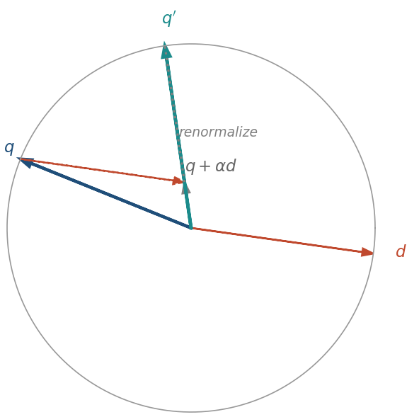
This is not equivalent to boosting candidates after retrieval. The query is edited first, and the new representation is used to search the index.
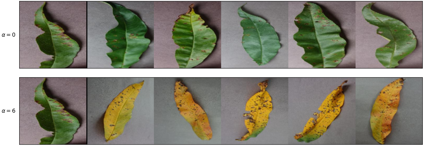
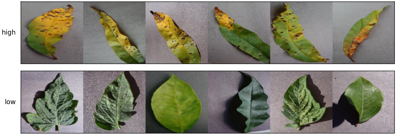
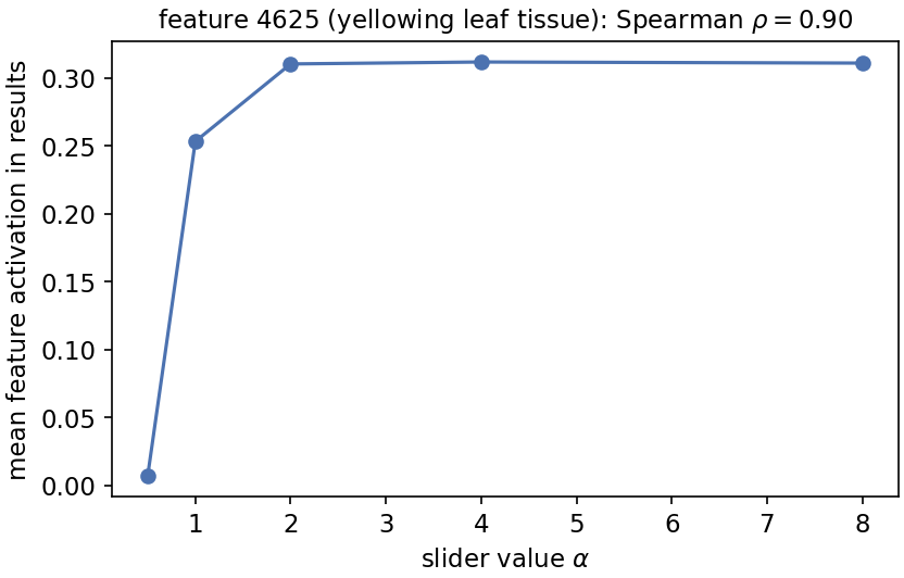
A useful slider should behave smoothly. For yellowing leaf tissue, the mean activation in retrieved results rose sharply between alpha = 0 and alpha = 2, then saturated. Its Spearman correlation between slider strength and retrieved activation was rho = 0.90.
With alpha = 0, the nearest results remain close to the original green query leaf. With alpha = 6, the ranking shifts toward yellow and damaged leaves while retaining the general object and structure of the query.
Why global nearest-neighbour search was not enough
A global embedding is fast and useful for broad similarity, but it weakens the relationship between a local feature and the result. A small brown lesion can be overwhelmed by overall shape, colour or background.
Patch-level retrieval addresses this with late interaction. Both the query and every corpus image are represented by sets of patch vectors. Candidate images are scored with MaxSim:
score(Q, C) = sum_j max_k similarity(q_j, c_k)
For each query patch q_j, the system finds the best matching corpus patch c_k. The 256 best-match similarities are then summed.
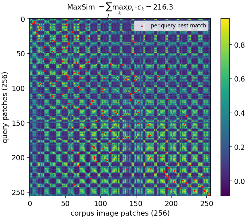
The matrix makes the computation visible. Every row corresponds to a query patch and every column to a corpus patch. The selected maximum in each row traces which region of the candidate image best explains each region of the query. In the inspected example, the MaxSim score was 216.3.

Steering is applied to the query patches before MaxSim retrieval. A direction associated with yellow tissue can modify the relevant local descriptors while the remaining patches continue to preserve shape, texture and context.
For larger corpora, FAISS first retrieves candidate patches, maps them back to image identifiers and computes exact MaxSim only for candidate images. The patch index can switch to IVF-PQ above a configurable size.
Dense similarity, sparse meaning
The original DINOv2 space remains the strongest source of general visual similarity. The SAE space is easier to interpret and contains the directions controlled by the sliders. SLIDERS can combine a dense FAISS index, an optional SAE-activation index and precomputed activation vectors for reranking.
The steering metrics are measured before the compensating reranker. Otherwise, a strong reranking rule could hide a weak feature direction and make the interface appear more faithful than the representation actually is.
Evaluating a steerable retrieval system
Standard retrieval metrics do not tell us whether a slider works. I therefore separated the evaluation into four additional properties.
Faithfulness measures whether steering increases the requested feature in the results relative to the unsteered baseline.
Isotonicity measures whether larger slider values produce larger effects, using Spearman correlation between alpha and the mean target activation.
Selectivity measures whether the target feature changes more than unrelated features.
Monosemanticity estimates whether a named unit repeatedly corresponds to the same visible pattern through the purity of its top-activating patches.
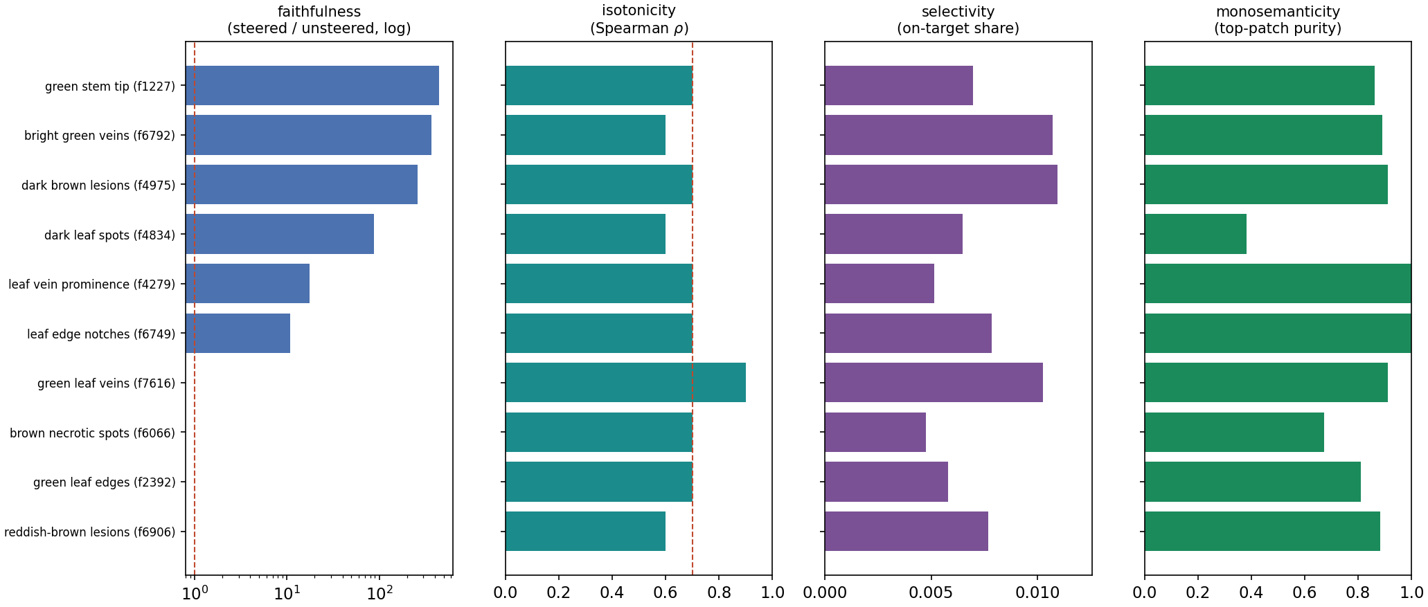
These metrics reveal trade-offs that recall and precision miss. A feature can be visually coherent but too weak to move the ranking. Another can move the ranking strongly but affect several concepts at once.
What the interface contributes
The frontend exposes the pieces needed to inspect the model: query upload, positive and negative steering, strongest and weakest examples, combinations of axes, full-resolution result inspection and reset controls.
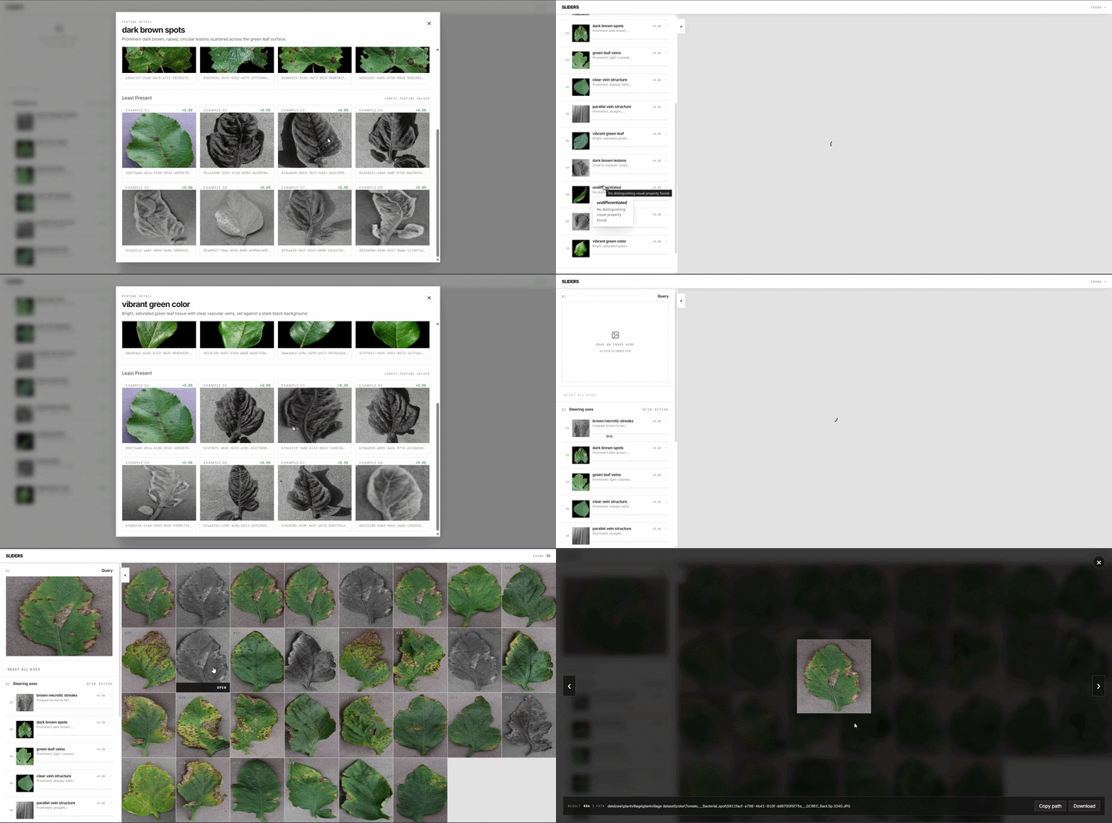
FastAPI serves the retrieval endpoints and static frontend. At startup, the application loads the encoder, SAE checkpoint, feature names, image paths, activation matrices and FAISS indexes into shared state.
Where the project stands
SLIDERS does not prove that every sparse visual feature is automatically a good user control. Some units remain mixed, some names are more reliable than others and large slider values can saturate. Patch-level retrieval also increases storage and computation compared with one-vector-per-image search.
What the project provides is a complete path from representation to interaction:
images
  -> DINOv2 patch tokens
  -> Sparse Autoencoder
  -> local feature evidence
  -> VLM feature names
  -> decoder directions
  -> query steering
  -> MaxSim retrieval
  -> faithfulness and interpretability metrics
The same sparse feature is used in three places: it activates on local evidence, it receives a name from that evidence and its decoder direction edits the query. That shared object is what connects the model to the interface.